
Assembling Chromatograms Tutorial
Learn how to edit and assemble chromatograms including bulk trimming of poor-quality sequences, editing sequences from alignments or assemblies, finding heterozygote and incorrectly called bases, and building consensus sequences from forward and reverse reads of the same gene.
Introduction
In this tutorial, you will take typical raw sequence data from a Sanger sequencing run and learn how to edit and align chromatograms for downstream analyses, such as building a phylogenetic tree or calculating nucleotide diversity.
The tutorial covers bulk trimming of poor-quality sequences, editing sequences from alignments or assemblies, finding heterozygote and incorrectly called bases, and building consensus sequences from forward and reverse reads of the same gene.
This tutorial requires the installation of the Heterozygotes plugin. To install this, go to Tools->Plugins, find it in the list of available Plugins and click Install.
INSTRUCTIONS
To complete the tutorial yourself with included sequence data, download the tutorial and install it by dragging and dropping the zip file into Geneious Prime. Do not unzip the tutorial.
THE DATASET
Mitochondrial DNA sequences dataset
EXERCISE 1
Editing mitochondrial DNA sequences
EXERCISE 2
Handling bidirectional nuclear sequence data

Mitochondrial DNA sequences – Introduction
The blue tit species complex includes C. caeruleus, found throughout Europe, C. teneriffae, found in North Africa and the Canary Islands, and C. cyanus, found in Asia and eastern Europe. Mitochondrial DNA data can be used to investigate the phylogeography and population structure of these species.
The dataset provided here comprises 34 sequences from the mitochondrial DNA control region of C. caeruleus and C. teneriffae. A sequence from the great tit Parus major is also included, as this would be a suitable outgroup for phylogenetic analysis.
The table below gives sampling location and codes for the sequences in this tutorial
| Code | Species | Origin |
| CEH | C. teneriffae | Canary Islands – El Hierro |
| CFU | C. teneriffae | Canary Islands – Fuerteventura |
| CGC | C. teneriffae | Canary Islands – Gran Canaria |
| CLG | C. teneriffae | Canary Islands – La Gomera |
| CLP | C. teneriffae | Canary Islands – La Palma |
| CLA | C. teneriffae | Canary Islands – Lanzarote |
| CTE | C. teneriffae | Canary Islands – Tenerife |
| MCE | C. teneriffae | Morocco – Ceuta |
| ECA | C. caeruleus | Spain – Cadiz |
| SRE | C. caeruleus | Sweden – Revinge |
| GB | C. caeruleus | Great Britain – Oxford |
| Pmaj | P. major | Sweden – Kvismaren |
Exercise 1: Editing Mitochondrial DNA sequences
Select the sequence list containing the raw sequence data from the mitochondrial DNA control region. Double-click on the list to open it in a new window. In the General tab to the right of the sequence view, choose to display Colors according to Quality. This will highlight the base calls according to the quality of the sequence at that base – the darker the blue, the lower the quality.
When zoomed out you won’t see the individual bases or chromatogram peaks, but there will be a graph visible giving an indication of sequence quality. If you scroll down the sequences you’ll see that the sequence quality decreases dramatically at the end of each sequence. Zoom in to at least 50% to see what the chromatograms look like in good vs poor quality regions. One of the sequences (CLG3) has no sequence, indicating the sequencing reaction failed so delete this one from the list. Sequence SRE1 has only a short stretch of good quality sequence before the sequence becomes unreadable so delete this one as well. Save the edited sequence list and close the window.
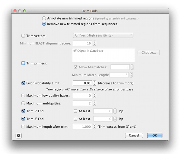
Trim the poor quality bases off the ends of the sequences by clicking Annotate and Predict→Trim Ends. Choose to “Remove new trimmed regions from sequences” and set the Error probability limit to 0.01, as shown in the screenshot below. Click OK and then Save once the trimming is finished.
From here it is more efficient to finish cleaning up and editing the sequences once they are aligned. Select the sequence list (Cyanistes CR sequences) again and click Align/Assemble→Multiple Align. Select the MUSCLE alignment algorithm and run it with the default settings.
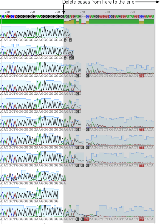
Double-click on the alignment to open it and zoom in to about 50% so you can see the base calls and chromatograms. You may need to check Show Graphs in the Graphs tab in order to see the chromatograms. Scroll along to the bases at the 3′ end and you’ll see that the base calls become weak after the GGGGGGGGAAGGGGGGGGG motif (see screenshot below). In many of the sequences the region following this motif is already trimmed off. Trim the remaining sequences by clicking Allow Editing then selecting the bases from base 563 onwards on the consensus sequence and hitting the delete key. Editing the consensus sequence will apply the change to all the sequences in the alignment. You should also delete the first 20 bases at the start of the alignment to make the sequences all the same length, as this region has already been trimmed off in a number of the sequences.
Click Save and choose Yes when asked if you want to apply the changes to the original sequences. Note that sometimes it is preferable not to apply the changes to the original sequences if you want to retain the original raw data file.
This alignment can now be used to build a phylogenetic tree of these sequences using the Tree function in Geneious. For more information on building and interpreting phylogenetic trees, see the Geneious phylogenetic analysis tutorials available from our website.
Exercise 2: Handling bidirectional nuclear sequence data
This exercise will give you more practice handling and editing raw sequence data produced by Sanger sequencing.
The Acrocephalus sequence list contains forward and reverse sequences for a nuclear gene from 3 different Acrocephalus reed warbler species. The sequences are named with a three-letter code to indicate their species (aru = A. arundinaceus, great reed warbler; dum = A. dumetorum, Blyth’s reed warbler; ort = A. orientalis, Oriental reed warbler), and are marked with ‘F’ or ‘R’ to indicate whether they were sequenced with forward or reverse primers.
Double-click on the Acrocephalus sequences list to open it in a new window. Scroll down to get an overview of the sequences. Note that in a few sequences the sequence quality drops off part way along (e.g. dum2 and dum4 sequences).
Trim the poor quality sequence off the ends of the sequence by clicking Annotate and Predict→Trim Ends. This time we will annotate the trimmed regions rather than deleting them altogether, so select “Annotate new trimmed regions”. Set the Error probability limit to 0.01 and click OK. Save the sequence list once the trimming is finished and close the sequence list window.
We now need to extract the sequence files from the list in order to set the read direction and use the heterozygote finder, as these options don’t work on sequence lists. Select the Acrocephalus sequence list and click Sequence→Extract Sequences from List. Choose to save the sequences in a subfolder called Acrocephalus Sequences.
We will now run the Heterozygote Finder on the individual sequence files to identify and annotate bases where two different nucleotides have been called at the same position. As these are nuclear sequences each represents two alleles, so there could be heterozygous positions where the two alleles have different bases and a double chromatogram peak is present. Select all the files in the Acrocephalus Sequences folder and click Annotate and Predict→Find Heterozygotes. Uncheck Search in Trimmed Regions, as regions where the sequence quality is poor will not give accurate results. Set the Peak Similarity to 50%, and choose to Annotate the heterozygote bases.
Click OK and Save the sequences when the analysis has finished. We will come back to the bases which are annotated as heterozygotes after we have assembled the forward and reverse sequences.
We will now assemble the forward and reverse sequences for each individual. To ensure that the sequences are assembled in the same orientation for each pair we first need to set the read direction. Holding down the command/cntrl key, select all the forward sequences in the folder (named with an F as the final letter), and select Sequence→Set Read Direction. Check the Forward box and click OK. There is no need to set the direction of the reverse reads as well.
Now select all the sequences in the folder and choose Align/Assemble→De Novo Assemble. Click Assemble by, then select 1st part of name, separated by underscore. This will produce one contig for each pair of forward and reverse sequences. Set the sensitivity to Highest Sensitivity/Slow, and ensure Save assembly report, Save list of unused reads, Save in sub-folder and Save contigs are checked. Choose to Use existing trim regions – with this option the assembler will ignore the regions annotated as trimmed, but you will still be able to see these regions on the sequences. Click OK.
A subfolder called Assembly has now been created which contains the contigs and an Assembly Report. You’ll also see a sequence list of unused reads, which contains sequences that could not be assembled. Take a look in this sequence list and you’ll see that these sequences are the ones which contained only a short stretch of good quality sequence (dum2 and dum4).
Exercise 2b: Checking assemblies and extracting the consensus
Open the aru2 contig from your Assembly subfolder to see how the forward and reverse sequences have assembled.
Under the Display tab to the right of the sequence viewer, check the options for calling the consensus sequence. When assembling forward and reverse sequences from the same gene, it makes sense to call the consensus from the sequence of the highest quality at each base, so select Highest Quality under Consensus.
Under the Advanced tab, set Base numbers to All sequences. This will display the base numbering from the original sequence reads on each sequence and enable you to see how the two sequences have assembled. You can see that the R sequence is now in the reverse orientation.
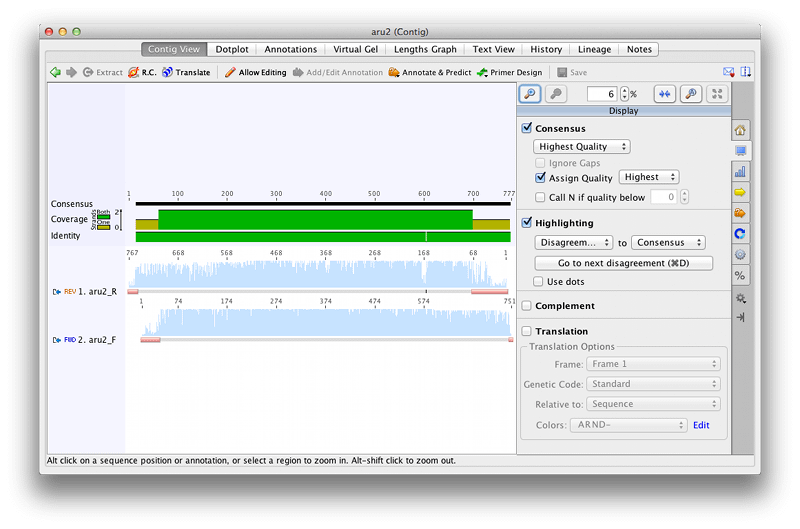
Under the Graphs tab, check the Coverage and Identity boxes. The Coverage Graph shows how many sequences the consensus sequence is based on, and the Identity Graph indicates whether the contributing sequences are identical or not. Although you can still see the poor quality sequence which has been annotated as trimmed (pink bars), you can see that the assembler has not used this sequence in calling the consensus sequence or calculating the coverage – only the single good sequence in this region has been used.
For Aru2 there is only a single base where there is a disagreement between the forward and reverse sequences. Zoom in and find this base. You can use the cntrl/command D keyboard shortcut to quickly jump to bases where there are disagreements. At this position the base in the reverse sequence has been called incorrectly – it should be an A but has been called as a C.
You can edit the errant sequence call at this position if you wish, but as we have chosen to call the consensus sequence based on the highest quality the base in the consensus sequence is correct. It is the consensus sequence that is used for downstream analyses so it is not necessary to edit every disagreement in the individual reads if the consensus is correct. Select the Consensus sequence and click Extract. Name your extracted sequence (e.g. aru2 consensus) and click OK.
Now open the ort1 assembly. This sequence has several heterozygous bases annotated which should be checked to ensure they have been called correctly. Click on the first heterozygous annotation on the ort1_R sequence (at base 68 on the consensus) and zoom into 100%. At this base, the single “G” peak has been called correctly so this has been incorrectly identified as a heterozygous base because of a small overlap with the adjacent “C” base. Remove this annotation by right-clicking on it and choosing Annotation→Delete.
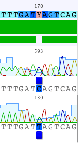
Now jump to the next heterozygous base using cntrl/command-D. At this base (position 170 on the Consensus sequence) there is a genuine double peak in both the forward and reverse reads where a C and a T peak are superimposed on top of each other, indicating that this is a real heterozygous base. The base called in the consensus sequence should be a “Y” indicating that this position contains both C and T nucleotides (see IUPAC Notation).
Now check the remaining heterozygous bases in this assembly and edit the consensus sequence by adding IUPAC ambiguity codes if required to reflect the heterozygous positions. Don’t forget to click Allow Editing before attempting to make any changes. Save your changes and choose Yes when asked if you want to apply the changes to the original sequences, then select the consensus sequence and Extract it.
Open each one of the other contigs and check for disagreements between the forward and reverse reads and heterozygote bases. Edit them if required, then extract the consensus sequence for each one.
Exercise 2c: Assembling to Reference
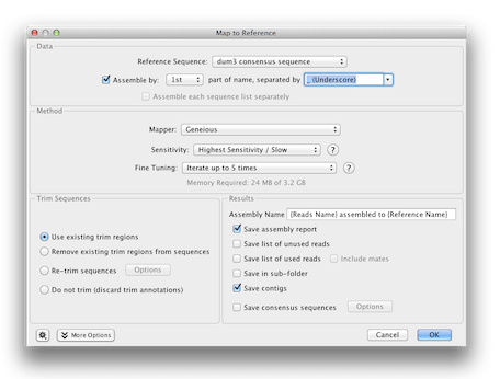
In order to assemble the two A. dumetorum sequences that did not work previously (because the overlapping parts of the sequence were poor quality and were trimmed off), we will assemble the partial sequences against a reference. Click on the Unused Reads sequence list from your Assembly, and holding down the control/command key click the dum3 consensus sequence, which we will use as a reference. Click Align/Assemble→Map to Reference. Ensure that the dum3 consensus sequence is set as the reference, and choose Assemble by, then select 1st part of name, separated by underscore. Set the other options as in the screenshot below.
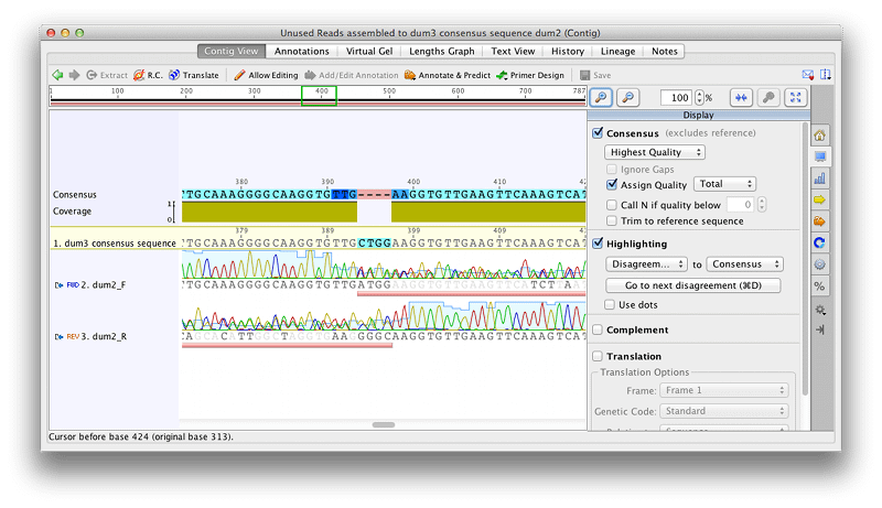
You should now have two new contig assemblies, one for dum2 and one for dum4. Open the dum2 assembly. You should now be able to see why these didn’t assemble using de-novo assembly, as there is a region of 4 bp where there is no good quality sequence that overlaps between the F and R sequences. A region of double peaks, which has been trimmed in both sequences, begins here – this is likely to represent an indel, where one of the two alleles contains a deletion.
Add an annotation to the consensus sequence to highlight the indel by selecting the 4 bp gap in the consensus sequence and clicking Add Annotation. Set the annotation type to Polymorphism, and name to Indel. Click OK and you should now see this annotation added to the consensus sequence. Click Save then extract the dum2 consensus sequence to a new file.
Repeat this process for the other reference assembly containing the dum4 sequences.
Exercise 2d: Analysing Consensus Sequences
You should now have produced consensus sequences for all 9 of the samples. These sequences can be aligned so that they can be used for population genetic or phylogenetic analyses. Select all the consensus sequences and click Align/Assemble→Multiple Align. Use the Geneious Aligner with the default settings.
Open the alignment and click on the Distances tab to get an overview of the nucleotide diversity within and between species. As you would expect, sequences are more similar within species than between species. In fact the sequences from A. arundinaceus (aru) are identical. You could now use the Tree building tools within Geneious to conduct a phylogenetic analysis of the sequences, or for more advanced population genetic analyses, the alignment can be exported in Fasta or Nexus format for analysis in a program such as DNAsp.
This concludes the Advanced Chromatograms Tutorial